ISA Atmosphäre als Funktion

Die Normatmosphäre, Normalatmosphäre oder Standardatmosphäre ist ein Begriff aus der Luftfahrt und bezeichnet idealisierte Eigenschaften der Erdatmosphäre.
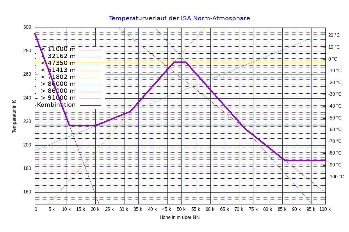
Die ICAO (International Civil Aviation Organization) hat 1976 mit ICAO-Dokument 7488[1] für die Luftfahrt eine allgemein gültige und verbindliche Normatmosphäre definiert. Der Temperaturverlauf mit der Höhe wird einer Tabelle definiert. Diese bilden also einzelne Funktionen die sich mit gnuplot einfach in eine einzige zusammanfassen lassen.
Graph des Luftdrucks und der Temperatur der ISA Atmosphäre
Skript-Download
#!/usr/bin/gnuplot
#   Modell für die Normalatmosphäre ISA (ISO2533:1975)
#
#    Geltungsbereich: bezogen auf geometrische Höhenangabe ü.N.N
#   Die Norm unterteilt die Funktion in mehrere Teile und hält die Daten in einer umfangreichen Tabelle fest.
#   Dies ist ein Modell das mit Formeln die Daten dieser Tabelle in eine einzige, 
#   einfach zu benutzende Funktion für die Temperatur und den Druck in Abhängigkeit der Höhe abbildet.
#
   Pnn = 101325.0   # Normaldruck in Pa
   Tnn = 288.15     # Normaltemperatur in K (=15 °C)
    r0 = 6.356766e6
 Tzero = -273.15

 T0(h) =  Tnn - 0.0065 * h    # Standard (in K)
 P0(h) = Pnn * (1.0 - h/44329)**5.255876
   Lh0 = 11000.0

  T1(h) = -Tzero - 56.5                           # Standard in K
  P1(h) = 22632*exp(1.73 - 0.000157*h)
    Lh1 = 20000.0

  T2(h) = -Tzero - 76.36349549 + 0.000991818 * h
  P2(h) = Pnn*0.223*exp((11019-h)/6470.0)
    Lh2 = 32162.0

  T3(h) = -Tzero  - 133.4035422 + 0.002765341 * h
  P3(h) = Pnn*(0.996 + h/209000)**-34.16319
    Lh3 = 47350.0

  T4(h) = -Tzero - 2.4646
  P4(h) = Pnn*(0.898309+h/55280)**-12.20114
    Lh4 = 51413.0

  T5(h) = -Tzero + 138.7452203 - 0.002746579 * h
  P5(h) = Pnn*0.00109456*exp((46998-h)/7922)
    Lh5 = 71802.0

  T6(h) = -Tzero + 81.61954906 - 0.001950979 * h
  P6(h) = Pnn*(0.838263-h/176142)**12.20114
    Lh6 = 86000.0

  T7(h) = 186.8673                    # in K, gültig  86km…91km
    Lh7 = 86000

  T8(h) = 263.1905-76.3232*((1.0-(h-91000)/-19.9429)**2)**0.5   # gültig  91km…110km
    Lh8 = 91000

  T9(h) = 240.0 + 12.0*(h-110000)     #  110km…120km
    Lh9 = 110000

 T10(h) = 1000 - (1000-360)*exp(-0.01875*(h-120000)*(r0+120000)/(r0+h))      #  120km…1000km
   Lh10 = 120000
#
#  Zusammengefasst in jeweils eine Funktion für Temperatur und Druck
T(h)  =  h<Lh0 ? T0(h) : h<Lh1 ? T1(h) : h<Lh2 ? T2(h) : h<Lh3 ? T3(h) : h<Lh4 ? T4(h) : h<Lh5 ? T5(h) : h<Lh6 ? T6(h) : T7(h)
P(h)  =  h<Lh0 ? P0(h) : h<Lh1 ? P1(h) : h<Lh2 ? P2(h) : h<Lh3 ? P3(h) : h<Lh4 ? P4(h) : h<Lh5 ? P5(h) : h<Lh6 ? P6(h) : T10(h)

set terminal pdf size 29.7cm,21cm
set output 'Atmosphere1.pdf'

set border
set key at screen 0.3,0.8 font "(,16)"
set xtics 5000
set mytics 10
set style line 51 lt 0 dt 1 lc rgb 'black'
set style line 52 lt 4 dt 3 lc rgb 'blue'
set grid ytics mytics xtics mxtics ls 52, ls 51     # Verschiedene Farben für die Gitter
set samples 1000
set format x "%.0s %c"
set lmargin 12; set rmargin 8; set tmargin 5; set bmargin 5
set xrange [-1000.0:100000.0]
set yrange [150:300]
set title "Temperaturverlauf der ISA Norm-Atmosphäre" font "(,16)" tc rgb 'blue'
set xlabel "Höhe in m über NN"
set ylabel "Temperatur in K"
set y2tics ( 1 )
do for [i=-100:30:10] {
    set y2tics add ( sprintf("%1.0f °C",i) i+273)
}
set multiplot
plot T0(x) title sprintf("< %.0f m",Lh0),\
     T1(x) title sprintf("< %.0f m",Lh2),\
     T2(x) title sprintf("< %.0f m",Lh3),\
     T3(x) title sprintf("< %.0f m",Lh4),\
     T4(x) title sprintf("< %.0f m",Lh5),\
     T5(x) title sprintf("> %.0f m",Lh6),\
     T6(x) title sprintf("> %.0f m",Lh7),\
     T7(x) title sprintf("> %.0f m",Lh8),\
      T(x) title "Kombination" lw 4
unset multiplot
set terminal png size 1200,800
set output 'Atmosphere-ISA1.png'
replot
set terminal pdf size 29.7cm,21cm
set output 'Atmosphere2.pdf'
set rmargin 12
unset yrange
#
set multiplot
set key at screen 0.3,0.4
set title "Druckverlauf der NormAtmosphäre, Tabellenwerte und kombinierte Abschnittsfunktionen" font "(,16)"
set ylabel "Druck in Pa"
set format y "%.0s %c"
unset y2tics
set xrange [-1000:70000.0]
set logscale y
set logscale y2
set yrange [10:120000]
set y2range [10:120000]
set y2label "mBar"
# add ytics from a list, as with log scale the "inc" operator is not useful
Asize=15
array TicList[Asize]=[40, 60, 200, 300, 400, 600, 2000, 3000, 4000, 6000, 20000, 30000, 40000, 60000, 80000]
do for [x=1:Asize] {
    set ytics add (TicList[x] TicList[x])
}
# add secondary scale with mBar units
Asize=11
array TicList[Asize]=[1000, 2000, 3000, 4000, 6000, 20000, 30000, 40000, 60000, 80000, 100000]
do for [x=1:Asize] {
    set y2tics add (sprintf("%.0f",TicList[x]/100) TicList[x])
}
plot  P(x) title "Kombination" lw 3, \
     P0(x) title sprintf("< %.0f m",Lh0), \
     P1(x) title sprintf("< %.0f m",Lh1), \
     P2(x) title sprintf("< %.0f m",Lh2), \
     P3(x) title sprintf("< %.0f m",Lh3), \
     P4(x) title sprintf("< %.0f m",Lh4), \
     P5(x) title sprintf("< %.0f m",Lh5), \
     'ISA.csv' using 1:2 with points title "Tabellenwerte der Norm"
#
unset xlabel
unset ylabel
unset key
unset title
set bmargin 0
set origin 0.48,0.49
set size 0.46,0.5
set object rectangle from screen 0.52,0.46 to screen 0.92,0.93 fillcolor rgb 'white' fillstyle solid behind
set xrange [-1000:10000.0]
set yrange [20000:120000]
set y2range [20000:120000]
set y2label "mBar"
set xtics 1000
set ytics add (20000 20000, 30000 30000, 40000 40000, 50000 50000, 60000 60000, 70000 70000)
plot  P(x) title "Kombination" lw 3, \
     P0(x) title sprintf("< %.0f m",Lh0), \
     P1(x) title sprintf("< %.0f m",Lh1), \
     P2(x) title sprintf("< %.0f m",Lh2), \
     P3(x) title sprintf("< %.0f m",Lh3), \
     P4(x) title sprintf("< %.0f m",Lh4), \
     P5(x) title sprintf("< %.0f m",Lh5), \
     'ISA.csv' using 1:2 with points title "Tabellenwerte der Norm"

unset multiplot
set terminal png size 1200,800
set output 'Atmosphere-ISA2.png'
replot
set output